Advanced Excel, Excel
Apr 23, 2026
How to Calculate Percentage in Excel
You can calculate percentages in Excel using basic multiplication and division. Whether you need to find a percentage of total, measure percentage change or calculate a specific percentage of a number, the formulas are straightforward. I'll show you how to use each one to make quick work of common percentage tasks in Excel.
Key Takeaways
- The basic percentage formula in Excel is =Part/Total. Format the result as a percentage using the Percent Style button or Ctrl+Shift+%.
- Use absolute references (e.g., $B$18) when calculating a column of percentages against a fixed total so the formula copies correctly.
- To calculate percentage change between two values, use the formula =(New Value-Old Value)/Old Value.
- To find a specific percentage of a number (e.g., 20% of a total), multiply the number by the decimal equivalent: =A1*0.20 or =A1*20%.
What Is the Percentage Formula in Excel?
Excel does not have a built-in PERCENTAGE function. Instead you use simple division or multiplication and then apply percentage formatting to the result. The core percentage formula looks like this:
=Part/Total
When you enter this formula, Excel returns a decimal (for example, 0.75 instead of 75%). You then format the cell as a percentage so the value displays the way you expect. This article covers three common scenarios:
| Scenario | Formula | Example |
|---|---|---|
| Percentage of total | =Part/Total | =B5/B18 |
| Percentage change | =(New-Old)/Old | =(650-500)/500 |
| Percentage of a number | =Number*Percentage | =A1*0.20 |
In the example below, column B shows travel expenses for the year and a yearly total (using the SUM function). In column C, we want to know the percentage that each month contributed to the total. Think of a pie chart: the total in B18 is the whole pie, and the percentages in column C will be the slices.

How to Format Cells as Percentages in Excel
Before diving into formulas, it helps to understand how Excel handles percentage formatting. When a formula returns 0.75, Excel displays exactly that until you tell it otherwise. Here is how to format cells as percentages:
- Select the cell or range you want to format.
- Click the Percent Style button on the Home tab of the Ribbon bar, or press Ctrl+Shift+% on your keyboard.
- Use the Increase Decimal or Decrease Decimal buttons on the Ribbon bar to control how many decimal places display.
One important detail: if a cell is already formatted as a percentage and you type 75, Excel interprets that as 7,500%. If you want 75%, either type 0.75 into a percentage-formatted cell or type 75 into an unformatted cell and then apply Percent Style afterward.
How to Calculate Percentage of Total in Excel
In C5, this formula divides the January amount by the total:
=B5/B18
But I won't enter it, yet! In order to save time and minimize data entry, I want to auto-fill the formula down to row 18. This will change the numerators (January through December), but leave the denominator fixed on B18 because I want to show each month divided by the same total.
To do this, I'll make the denominator an absolute reference by clicking it and pressing the F4 key on the keyboard. That makes the formula look like this:
=B5/$B$18
Tip: $B tells Excel to not rewrite the columns when I fill, and $18 tells Excel not to rewrite the rows. Since you are filling straight down column C, the column letter B would not shift regardless. However, adding the dollar sign before both the column and row is good practice for consistency.
Now I'll enter the formula, but the result is a decimal:

Instead of showing this long decimal, I want a percentage and I want to round it off after two digits. This takes just one click:
Select the long decimal in C5, then click the Percent Style butto  n on theHome tab of the Ribbon bar.
Tip: To increase or decrease the number of decimal places showing, click the Increase Decimal or Decrease Decimal button on the Ribbon bar.
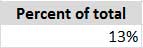
This gives me the percent that I want:
Now I’ll auto-fill the formula down to row 18. When you click any cell, do you notice the small dot in the lower-right corner?

When you roll the mouse over the dot, the mouse pointer becomes a crosshair.

Now I’ll drag the crosshair downwards:

Now the entire column is filled with percentages (I deleted the zero in C17). Once your percentages are in place, you can use conditional formatting to automatically highlight months that exceed a threshold, making it easy to spot where spending was highest.

If you'd like to examine this worksheet, download Percentage Formula 1_travel expenses.xlsx. You can test yourself by deleting all the numbers down column C and trying it on your own.
How to Calculate Percentage Increase or Decrease in Excel
Another common task is measuring how much a value has changed over time. The percentage change formula in Excel is:
=(New Value-Old Value)/Old Value
For example, suppose your sales were $500 in January and $650 in February. To calculate the percentage increase:
- In a new cell, enter =($650-$500)/$500 or reference the cells directly, such as =(B2-B1)/B1.
- Excel returns 0.3, which is a decimal.
- Apply Percent Style to display the result as 30%.
A positive result means an increase. A negative result means a decrease. If February sales dropped to $400 instead, the formula would return -20%, telling you sales fell by that amount.
When you need to calculate percentage change across an entire column, use an absolute reference on the baseline value (the "old" value) if every row compares back to the same starting number. If each row compares to the row above it, relative references work fine.
How to Find a Specific Percentage of a Number in Excel
Sometimes you need to calculate a specific percentage of a value, such as a 20% discount or an 8% tax. The formula is simple multiplication:
=Number*Percentage
For example, to find 20% of $1,500, enter:
=1500*0.20
Or you can use the percent symbol directly:
=1500*20%
Both formulas return 300. Excel recognizes the % symbol and converts 20% to 0.20 automatically.
This approach works for any scenario where you need a portion of a value: sales tax, tip calculations, budget allocations or discount amounts. If you regularly work with financial data, Excel finance formulas can take these calculations even further. Just replace the percentage with whatever rate you need.
Common Percentage Errors and How to Fix Them
If your percentage results look wrong, you are likely running into one of these common issues:
- Result shows 7500% instead of 75%. This happens when the cell is already formatted as a percentage before you enter a formula that returns a decimal. Excel multiplies the decimal by 100 again. To fix it, clear the cell formatting first (Home > Clear > Clear Formats), enter your formula and then apply Percent Style.
- Result shows 0%. Your formula is likely referencing empty cells or cells that contain text instead of numbers. Double-check that all referenced cells contain numeric values.
- #DIV/0! error. You are dividing by zero or by an empty cell. Make sure the denominator cell contains a value greater than zero. You can wrap your formula in an IFERROR function to display a friendlier message: =IFERROR(B5/$B$18, "N/A").
- Percentages don't add up to 100%. This is usually a rounding issue. Each individual percentage gets rounded, and the rounded values may not sum to exactly 100%. Use the ROUND function on each percentage to control precision, or accept a small variance as normal.
Sharpen Your Excel Skills with Pryor Learning
Percentage formulas are just one piece of building real confidence in Excel. Pryor Learning offers live and On-Demand Excel courses covering formulas, data analysis, pivot tables and more. Whether you are just getting started or looking to sharpen advanced skills, explore what is available through PryorPlus or individual seminars to keep building your expertise.


