Basic Excel, Excel
Jul 28, 2026
How to Find Duplicates in Excel and Remove Them
Key Takeaways
- Excel offers multiple ways to find duplicates, from visual highlighting with conditional formatting to formula-based detection with COUNTIF and automated cleanup with the Remove Duplicates feature.
- The best method depends on whether you need to identify, count, extract or remove duplicate values in your data.
- Always back up your data before removing duplicates, as the action is permanent and cannot be undone after saving.
- For large datasets, Power Query provides the most scalable and repeatable approach to deduplication.
Why Finding Duplicates in Excel Matters
It's a common scenario: Data is combined from multiple sources, records are entered by multiple users or you simply have multiple transactions with the same information. The end result is that you need to find and manipulate duplicates.
Duplicate data is more than a minor annoyance. When left unchecked, duplicate values in Excel can lead to inaccurate reports, skewed analysis and wasted resources. Imagine sending the same marketing mailer to a customer three times or double-counting revenue in a quarterly summary. These are real consequences that affect decisions and budgets.
Common causes of duplicates include merging spreadsheets from different departments, importing records from external systems, manual data entry by multiple team members and repeated form submissions. The larger your dataset, the more likely duplicates are hiding in it.
Excel gives you several ways to find and remove duplicates in Excel, depending on your data and what results you are after. This article covers seven methods and scenarios in which you might use them: conditional formatting, Advanced Filter, the built-in Remove Duplicates feature, COUNTIF formulas, the UNIQUE function, PivotTables and Power Query.
Finding vs. Removing Duplicates: Know What You Need
Before diving into specific methods, it helps to understand the difference between finding duplicates and removing them. Some approaches are non-destructive, while others permanently alter your data.
Non-destructive methods let you identify duplicates without changing your spreadsheet:
- Conditional formatting: Highlights duplicate cells with a color fill so you can visually scan your data
- COUNTIF formula: Flags duplicates in a helper column you can filter or sort
- UNIQUE function: Extracts a separate list of unique values, leaving the original data untouched
- PivotTable: Summarizes and counts duplicate entries for analysis
Destructive methods permanently remove rows from your dataset:
- Remove Duplicates feature: Deletes duplicate rows in place, keeping only the first occurrence
- Advanced Filter: Copies unique records to a new location (original data stays intact, but the filtered copy excludes duplicates)
- Power Query: Removes duplicate rows within a query that can be refreshed as source data changes
If you are unsure whether you need to keep certain duplicates, start with a non-destructive method to review your data before committing to deletion.
Use Conditional Formatting to Highlight Duplicates
Scenario: You have a spreadsheet of customer email addresses and want to quickly see which ones appear more than once before deciding what to do with them. Conditional formatting is the fastest way to visually spot duplicates without altering your data.
- Select the range of cells you want to check for duplicates. This can be a single column or multiple columns.
- On the Home tab, click Conditional Formatting in the Styles group.
- Choose Highlight Cells Rules, then select Duplicate Values.
- In the Duplicate Values dialog box, choose the formatting style you prefer (the default is a light red fill with dark red text) and click OK.
Excel will immediately highlight every cell in the selected range that contains a duplicate value. You can then scroll through your data to review the highlighted entries and decide whether to keep, edit or remove them.
Note: Conditional formatting highlights duplicates within the selected range only. If you need to compare values across different sheets or workbooks, use a formula-based approach like COUNTIF instead.
Use Advanced Filter
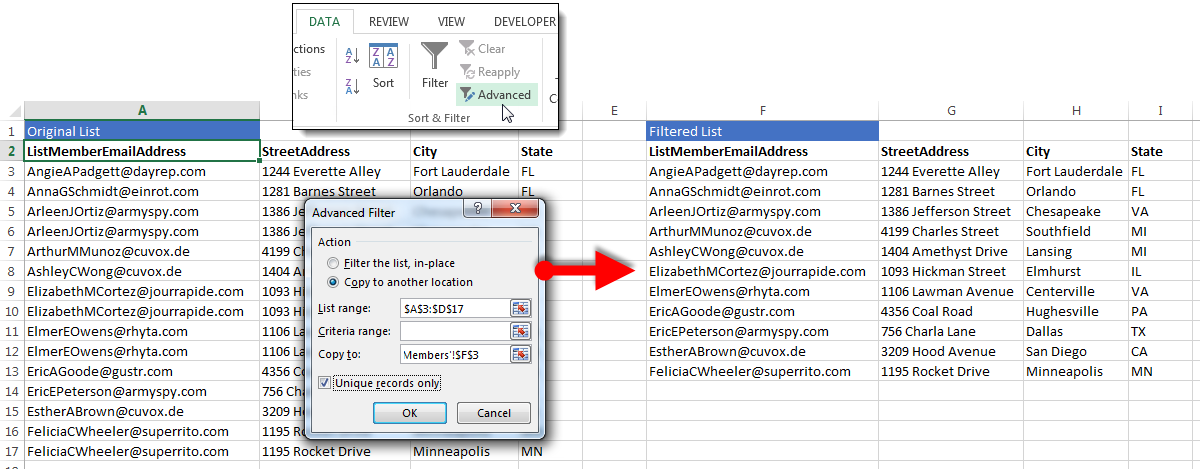
Scenario: We have a list of people who were members of our business association in one year, and another list of those who were members the following year. We would like to generate a new list of all people who were members in one or both years and remove the duplicate rows of the members who were in both. With the advanced filter we can do this in one step. To follow using our example, download Find Duplicates.xlsx: Renewing Members
Start by merging the two lists into a new sheet using copy/paste or Excel's Consolidate feature, etc. These steps work across modern versions of Excel, though the interface may look slightly different depending on your version.
- Click on any cell with data in your worksheet.
- Click the Advanced button in the Sort & Filter group on the Data tab.
- In the Advanced Filter dialog box:
- Choose the Copy to another location radio button
- Check to see that Excel has correctly identified the data you wish to filter in the List range: text box and select or correct the range if not
- Choose a destination for the filtered list in the Copy to box. This can be on the same sheet or in another sheet.
- Check Unique records only. This will copy all unique records and only 1 instance of any duplicated record.
Note: This method only removes duplicates when the entire row/record is the same. If you need to identify records that only have some fields in common, use the next method, Excel's Built-in Remove Duplicates Feature.
Use Excel's Built-in Remove Duplicates Feature
Scenario: We would like to mail a print postcard to the members of our email mailing list, but have discovered that some have signed up more than once with different email addresses. This means we would send multiple postcards to the same address. We want to remove those duplicate addresses.
Hint! Always start by creating a copy of your worksheet before you begin working so your original data remains safe.
To follow using our example, download Find Duplicates.xlsx: Mailing List
- Click on any cell with data in your worksheet.
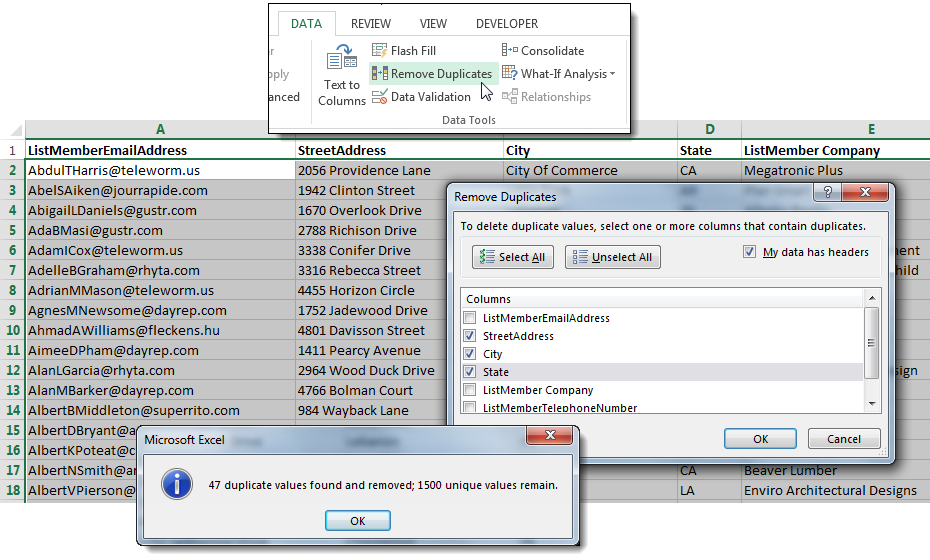
- On the Data tab, click Remove Duplicates to open the Remove Duplicates dialog box.
- Put a checkbox by each column that has duplicate information in it. In our example, we want to find identical addresses. (Note: Hit Select All to only remove records that are exactly alike.)
- Click OK. Excel will automatically find and remove all but the first row of matches that contain the same information.
Use the COUNTIF Function to Detect Duplicates
Scenario: You manage a spreadsheet of product SKUs submitted by multiple warehouse locations and suspect that some SKUs have been entered more than once. You want to flag every duplicate entry so you can review them before taking action.
The COUNTIF function lets you create a helper column that identifies duplicates without modifying your original data.
- In a blank column next to your data, add a header such as "Duplicate?" in the first row.
- In the first cell below your header (for example, cell B2 if your data is in column A), enter the formula: =COUNTIF($A$2:$A$100,A2)>1. Adjust the range to match your actual data.
- Press Enter. The formula returns TRUE if the value in that row appears more than once in the range, or FALSE if it is unique.
- Copy the formula down to fill the entire column alongside your data.
- To isolate the duplicates, click the filter arrow on your helper column header and filter for TRUE. You will now see only the rows that contain duplicate values.
From here you can review, correct or delete the flagged rows as needed. Because the helper column is separate from your original data, nothing is lost until you choose to make changes.
Tip: If you want to count exactly how many times each value appears, use =COUNTIF($A$2:$A$100,A2) without the >1 comparison. This returns the count as a number, which can be useful for spotting entries that appear three, four or more times.
Use the UNIQUE Function to Extract Unique Values
Scenario: You have a long list of vendor names collected from multiple purchase orders and need a clean, deduplicated list to update your vendor directory. Rather than modifying the original data, you want to generate a separate list of unique names automatically.
The UNIQUE function, available in Excel 365 and later versions, uses dynamic arrays to spill a list of unique values into adjacent cells.
- Click on an empty cell where you want the unique list to begin.
- Enter the formula: =UNIQUE(A2:A100). Adjust the range to match your data.
- Press Enter. Excel will automatically spill a list of unique values starting from that cell, with duplicates removed.
The result updates dynamically. If you add or change values in the source range, the unique list adjusts automatically.
To extract only values that appear exactly once (truly one-of-a-kind entries rather than the first instance of each value), use the formula: =UNIQUE(A2:A100,FALSE,TRUE). The third argument set to TRUE tells Excel to return only values with no duplicates at all.
Note: If you are using an older version of Excel that predates Excel 365, the UNIQUE function is not available. Use one of the other methods in this article, such as Advanced Filter or COUNTIF, to achieve similar results.
Use a PivotTable
Scenario: You have a spreadsheet listing all attendees at a convention you are hosting. You want to know how many people from each company are attending so you can offer a discount to those bringing 5 or more employees.
To get a count of rows that have duplicate information, in this case – the same company name – a PivotTable offers you a very quick way to view and then manipulate that information.
To follow using our example, download Find Duplicates.xlsx: PivotTable
1) Insert a new, blank PivotTable into your workbook.
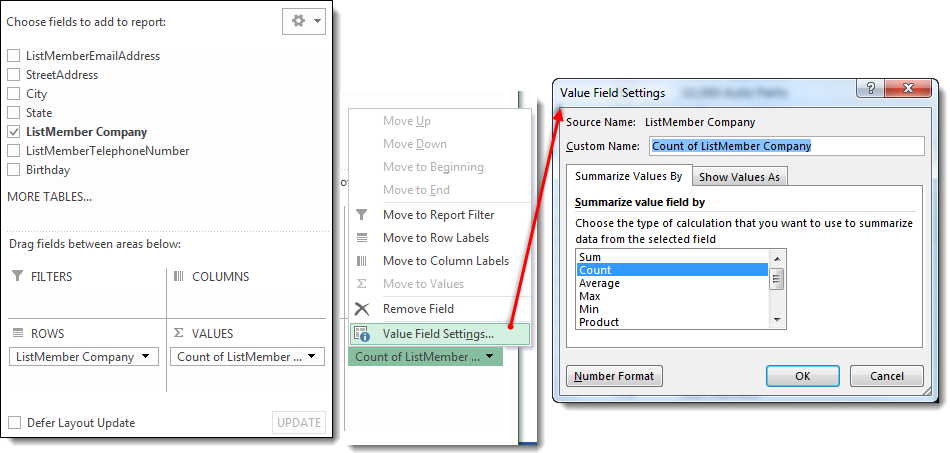
2) In the PivotTable Fields pane, choose the field that contains duplicates and place it both in the Rows area AND in the Values area. The Summarize setting should default to Count but if it does not, open the Value Field Settings dialog box and choose Count from the selection box. The result will be a PivotTable that shows each company in the left column and the number of times that company appears in the column in the right column. This is the number of attendees from each company.
3) Since we want to only see those companies that have 5 or more attendees, we will need to add a filtering step. Click on the filter arrow on the Row Labels header.
4) Choose Value Filters and then the appropriate criteria, in this case Greater Than Or Equal To.
5) Fill out the details of your criteria in the Value Filter dialog box and click OK.
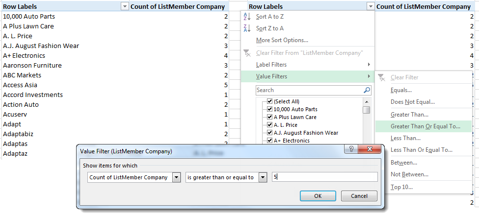
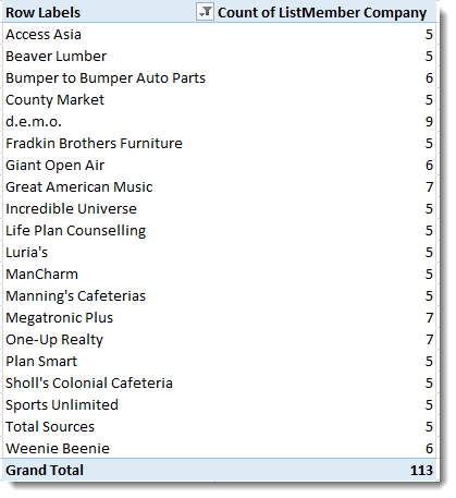
Our PivotTable will now only show those rows that have 5 or more duplicates in the ListMember Company column on the original table.
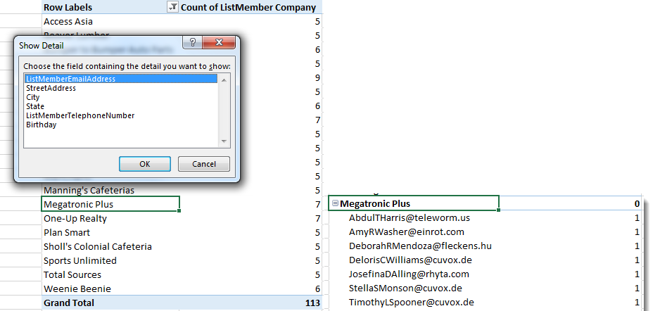
A very useful feature of a PivotTable is that you can then "drill down" into the data behind the summary. Double-click on any of the "5 or more" companies to see attendee detail for that company, for example. Techniques like these are covered in depth in advanced Excel PivotTable training.
Use Power Query for Large-Scale Deduplication
Scenario: You manage a transaction log with tens of thousands of rows imported monthly from multiple point-of-sale systems. Manual methods are too slow and you need a repeatable process that updates every time new data arrives.
Power Query, built into modern versions of Excel, provides a scalable way to remove duplicates within a structured query. Because the query saves your transformation steps, you can refresh it whenever the source data changes without repeating the work manually.
- Click on any cell in your data range, then go to the Data tab and click From Table/Range in the Get & Transform Data group. If your data is not already formatted as a table, Excel will prompt you to create one.
- The Power Query Editor will open with your data loaded. Select the column or columns you want to check for duplicates. To select multiple columns, hold Ctrl and click each column header.
- On the Home tab in the Power Query Editor, click Remove Rows, then choose Remove Duplicates.
- Power Query will remove all duplicate rows based on the selected columns, keeping only the first occurrence of each unique combination.
- Click Close & Load to send the cleaned data back to your workbook as a new table.
To refresh the results after your source data changes, right-click the query table in your workbook and select Refresh. Power Query will reapply all your transformation steps automatically.
Tip: Power Query also lets you merge data from multiple files or sources before deduplicating, making it ideal for consolidating records from different departments or systems in a single workflow.
Choosing the Right Method for Your Needs
With seven methods available, picking the right one depends on what you need to accomplish, how large your dataset is and which version of Excel you are using.
| Method | Best For | Destructive? | Skill Level | Excel Version |
|---|---|---|---|---|
| Conditional Formatting | Visually spotting duplicates in small to medium lists | No | Beginner | 2007+ |
| Advanced Filter | Copying unique records to a new location | No (copies data) | Intermediate | 2007+ |
| Remove Duplicates | Quickly deleting duplicate rows in place | Yes | Beginner | 2007+ |
| COUNTIF Formula | Flagging duplicates with a helper column for review | No | Beginner | 2007+ |
| UNIQUE Function | Generating a dynamic list of unique values | No | Beginner | 365 / 2021+ |
| PivotTable | Counting and analyzing duplicate entries | No | Intermediate | 2007+ |
| Power Query | Deduplicating large or recurring datasets | Yes (in query output) | Intermediate | 2016+ |
If you just need to visually scan for duplicates, start with conditional formatting. If you need to permanently clean a list with minimal effort, the Remove Duplicates feature is the fastest option. For formula-driven workflows where you want to review before deleting, COUNTIF gives you full control. And if you are working with large datasets that update regularly, Power Query saves time by making the process repeatable.
Best Practices for Managing Duplicates in Excel
No matter which method you choose, following a few best practices will help you avoid mistakes and protect your data.
- Always back up your data first: Before running any destructive operation like Remove Duplicates, save a copy of your original worksheet. Once duplicates are removed and the file is saved, there is no way to recover deleted rows.
- Use helper columns for non-destructive checks: A COUNTIF formula in a helper column lets you flag and review duplicates before deciding what to delete. This extra step can prevent accidental data loss.
- Watch for case sensitivity: Excel's built-in duplicate tools are not case-sensitive, meaning "Smith" and "smith" are treated as the same value. If case matters in your data, use a formula-based approach with the EXACT function.
- Trim leading and trailing spaces: Extra spaces can cause identical-looking values to be treated as unique. Use the TRIM function to clean your data before checking for duplicates.
- Check formatting consistency: Numbers stored as text and numbers stored as values may look the same but will not match as duplicates. Standardize formatting before deduplicating.
- Consider partial matches: Decide in advance whether records need to match on every field or only on specific columns. The Remove Duplicates feature lets you select which columns to compare.
- Test on a small sample first: If you are working with a large dataset, apply your chosen method to a small subset to confirm it produces the expected results before running it on the full file.
Build Your Excel Skills with Pryor Learning
Though you will have different data and different scenarios, one of the techniques above can help you get started on the solution you need when working with data that has duplicate information.
Finding and managing duplicates is just one of many essential Excel skills that can save you hours of manual work. Whether you are cleaning up a mailing list, reconciling financial records or preparing data for analysis, knowing which tool to reach for makes all the difference.
Pryor Learning offers hands-on Excel training designed for every skill level, from beginners learning the basics to experienced users looking to master advanced features. Training options include:
- Live seminars: Instructor-led sessions covering core and advanced Excel skills
- On-demand courses: Self-paced lessons you can take anytime, anywhere
- PryorPlus: Unlimited access to Pryor's full library of courses for ongoing professional development