Management, Supervision & Leadership
Jul 29, 2026
How to Freeze a Row in Excel

Key Takeaways:
- Freezing rows in Excel keeps headers and key data visible while you scroll through large spreadsheets.
- Use View > Freeze Panes to freeze the top row, the first column or multiple rows and columns at once.
- The cell you select before clicking Freeze Panes determines which rows and columns stay locked in place.
- You can unfreeze panes at any time from the same Freeze Panes dropdown on the View tab.
Freezing a row in Excel locks it in place so it stays visible as you scroll through your spreadsheet. This is essential when you are working with large datasets - Excel supports over 1 million rows and more than 16,000 columns of data. Without frozen rows, you would have to scroll back to the top every time you need to check a column header. Freezing rows and columns helps keep the information you need in view on the Excel window, and pairing this with hyperlinks in Excel can further streamline navigation in complex workbooks.
How to Use Freeze Panes in Excel
Excel's Freeze Panes feature, found on the View tab, offers three options: Freeze Top Row, Freeze First Column and Freeze Panes. Here are the steps for each method.
Freeze the Top Row
- Scroll until the row you want to remain "on top" is the very first row in the window.
- Click the View tab.
- Click the Freeze Panes dropdown.
- Click Freeze Top Row.

Now when you scroll up and down through your spreadsheet, the top row stays in place and the other rows pass under it.
Important Tip! Excel will freeze any row that is at the top of the window using this method. It is a common misunderstanding that only Row 1 freezes. If the row that is frozen is not Row 1, you will not be able to scroll higher than the frozen row! For example, if you freeze Row 21 as your top row, then you will not be able to see Rows 1-20 until you unfreeze it.
Freeze the First Column
- Scroll until the column you want to remain "on the left" is the very first column in the window.
- Click the View tab.
- Click the Freeze Panes dropdown.
- Click Freeze First Column.

Now when you scroll left and right through your spreadsheet, the left column stays in place and the others pass under it.
Important Tip! Excel will freeze any column that is leftmost in the window using this method. If the column that is frozen is not Column A, you will not be able to scroll past the frozen one! For example, if you freeze Column D as your first column, then you will not be able to see Column A-C until you unfreeze it.
Note that these two commands can not be used together. Clicking Freeze First Column will cancel a freeze on the first row, for example. So that leads us to the next question:
Freeze Multiple Rows and Columns
You can freeze multiple rows and columns at the same time, but it does take a little thinking to get your head around how it works. Here are the steps:
- Place your cursor in the cell to the right and/or below where you want the freezing lines to be drawn. Here are several examples of how to choose which cell you need:
- Click cell A2 to freeze the top row.
- Click cell B1 to freeze the first column.
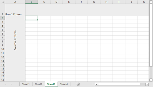
- Click cell B2 to freeze the top row and the left column. (See Image)
- Click cell C3 to freeze the top two rows and the left two columns.
- Click the View tab.
- Click the Freeze Panes dropdown.
- Click Freeze Panes.
Now when you scroll, any row above where your cursor was placed will remain in place and any column to the left of your cursor will be frozen. At first it can be tricky to figure out which cell to click to freeze the correct rows and columns, especially if you are still building your Excel basics. Try it a few times, freezing and unfreezing, until you get the hang of it.
The table below provides a quick reference for common freeze scenarios using Excel freeze panes.
| Cell Selected | Rows Frozen | Columns Frozen |
|---|---|---|
| A2 | Row 1 (top row) | None |
| B1 | None | Column A (first column) |
| B2 | Row 1 | Column A |
| C3 | Rows 1-2 | Columns A-B |
| D4 | Rows 1-3 | Columns A-C |
Troubleshooting Tips for Freeze Panes
Even experienced Excel users run into issues with freeze panes from time to time. Here are solutions to the most common problems:
- Wrong row frozen: Scroll so the desired row is at the top of the window before applying Freeze Top Row. If you want to freeze a specific row in Excel that is not Row 1, use the Freeze Panes option instead by selecting the cell in Column A directly below the last row you want frozen.
- Cannot scroll to rows above the frozen row: Unfreeze panes first, then scroll to the position you need and reapply the freeze.
- Freeze Panes option is grayed out: Check if you are in cell editing mode (press Escape to exit) or if the worksheet is protected. You must exit editing mode before the Freeze Panes dropdown becomes available.
- Want to freeze a row that is not Row 1: Use the Freeze Panes option (not Freeze Top Row). Click the cell in Column A directly below the last row you want frozen, then go to View > Freeze Panes > Freeze Panes.
- Midpoint freeze: Place your cursor in cell A1 and then follow the steps to freeze panes. This will tell Excel to freeze your sheet along vertical and horizontal midpoints.

How to Unfreeze Rows and Columns in Excel
Follow these steps to unfreeze rows and columns.
- Click the View tab.
- Click the Freeze Panes dropdown.
- Click Unfreeze Panes.

Unfreezing removes all frozen panes at once. You can then reapply a freeze in a different position as needed.
With this tool at your fingertips, you won't have to scroll back and forth to read headings or stretch your window from edge to edge of your monitor just to see the data you need to compare. Freeze a row to keep your headers in sight, apply conditional formatting to flag important values or freeze a specific record that you want to use as a basis of comparison for other records.